Hierarchical Networks
CodeSnippet
You can download all the code on this page from the code snippets directory
The hinet subpackage makes it possible to
construct arbitrary feed-forward architectures, and in particular
hierarchical networks (networks which are organized in layers).
Building blocks
The hinet package contains three basic building blocks, all of which are
derived from the Node class: Layer, FlowNode,
and Switchboard.
The first building block is the Layer node, which works like a
horizontal version of flow. It acts as a wrapper for a set of nodes
that are trained and executed in parallel. For example, we can
combine two nodes with 100 dimensional input to construct a layer
with a 200-dimensional input:
>>> node1 = mdp.nodes.PCANode(input_dim=100, output_dim=10)
>>> node2 = mdp.nodes.SFANode(input_dim=100, output_dim=20)
>>> layer = mdp.hinet.Layer([node1, node2])
>>> layer
Layer(input_dim=200, output_dim=30, dtype=None)
The first half of the 200 dimensional input data is then automatically
assigned to node1 and the second half to node2. A layer
Layer node can be trained and executed just like any other node.
Note that the dimensions of the nodes must be already set when the layer
is constructed.
In order to be able to build arbitrary feed-forward node structures,
hinet provides a wrapper class for flows (i.e., vertical stacks
of nodes) called FlowNode. For example, we can replace
node1 in the above example with a FlowNode:
>>> node1_1 = mdp.nodes.PCANode(input_dim=100, output_dim=50)
>>> node1_2 = mdp.nodes.SFANode(input_dim=50, output_dim=10)
>>> node1_flow = mdp.Flow([node1_1, node1_2])
>>> node1 = mdp.hinet.FlowNode(node1_flow)
>>> layer = mdp.hinet.Layer([node1, node2])
>>> layer
Layer(input_dim=200, output_dim=30, dtype=None)
In this example node1 has two training phases (one for each internal
node). Therefore layer now has two training phases as well and
behaves like any other node with two training phases. By combining and
nesting FlowNode and Layer, it is thus possible to build modular
node structures. Note that while the Flow interface looks pretty
similar to that of Node it is not compatible and therefore we must
use FlowNode as an adapter.
When implementing networks one might have to route different parts of
the data to different nodes in a layer. This functionality is provided
by the Switchboard node. A basic Switchboard is initialized with a 1-D
Array with one entry for each output connection, containing the
corresponding index of the input connection that it receives its input
from, e.g.:
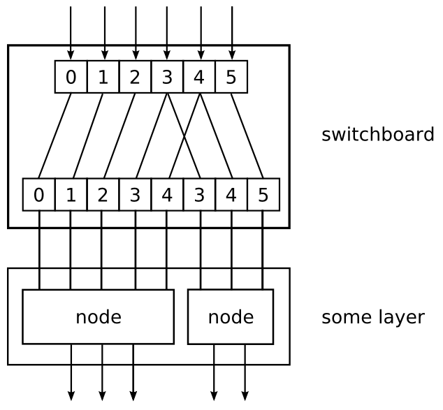
>>> switchboard = mdp.hinet.Switchboard(input_dim=6, connections=[0,1,2,3,4,3,4,5])
>>> switchboard
Switchboard(input_dim=6, output_dim=8, dtype=None)
>>> x = mdp.numx.array([[2,4,6,8,10,12]])
>>> switchboard.execute(x)
array([[ 2,  4,  6,  8, 10,  8, 10, 12]])
The switchboard can then be followed by a layer that splits the routed input to the appropriate nodes, as illustrated in following picture:
By combining layers with switchboards one can realize any
feed-forward network topology. Defining the switchboard routing
manually can be quite tedious. One way to automatize this is by
defining switchboard subclasses for special routing situations. The
Rectangular2dSwitchboard class is one such example and will be
briefly described in a later example.
HTML representation
Since hierarchical networks can be quite complicated, hinet
includes the class HiNetHTMLTranslator that translates
an MDP flow into a graphical visualization in an HTML file. We also provide
the helper function show_flow which creates a complete HTML file with
the flow visualization in it and opens it in your standard browser.
>>> mdp.hinet.show_flow(flow)
To integrate the HTML representation into your own custom HTML file
you can take a look at show_flow to learn the usage of
HiNetHTMLTranslator. You can also specify custom translations for
node types via the extension mechanism (e.g to define which parameters are
displayed).
Example application (2-D image data)
As promised we now present a more complicated example. We define the lowest layer for some kind of image processing system. The input data is assumed to consist of image sequences, with each image having a size of 50 by 50 pixels. We take color images, so after converting the images to one dimensional numpy arrays each pixel corresponds to three numeric values in the array, which the values just next to each other (one for each color channel).
The processing layer consists of many parallel units, which only see a
small image region with a size of 10 by 10 pixels. These so called
receptive fields cover the whole image and have an overlap of five
pixels. Note that the image data is represented as an 1-D
array. Therefore we need the Rectangular2dSwitchboard class to
correctly route the data for each receptive field to the corresponding
unit in the following layer. We also call the switchboard output for
a single receptive field an output channel and the three RGB values
for a single pixel form an input channel. Each processing unit is a
flow consisting of an SFANode (to somewhat reduce the
dimensionality) that is followed by an SFA2Node. Since we assume
that the statistics are similar in each receptive filed we actually
use the same nodes for each receptive field. Therefore we use a
CloneLayer instead of the standard Layer. Here is the actual
code:
>>> switchboard = mdp.hinet.Rectangular2dSwitchboard(in_channels_xy=(50, 50),
...                                                  field_channels_xy=(10, 10),
...                                                  field_spacing_xy=(5, 5),
...                                                  in_channel_dim=3)
>>> sfa_dim = 48
>>> sfa_node = mdp.nodes.SFANode(input_dim=switchboard.out_channel_dim,
...                              output_dim=sfa_dim)
>>> sfa2_dim = 32
>>> sfa2_node = mdp.nodes.SFA2Node(input_dim=sfa_dim,
...                                output_dim=sfa2_dim)
>>> flownode = mdp.hinet.FlowNode(mdp.Flow([sfa_node, sfa2_node]))
>>> sfa_layer = mdp.hinet.CloneLayer(flownode,
...                                  n_nodes=switchboard.output_channels)
>>> flow = mdp.Flow([switchboard, sfa_layer])
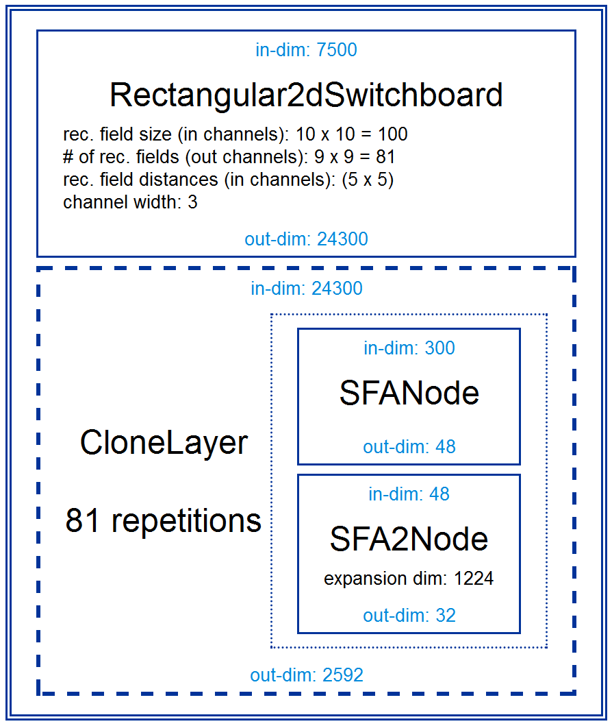
The HTML representation of the the constructed flow looks like this in your browser:
Now one can train this flow for example with image sequences from a movie.
After the training phase one can compute the image pattern that produces
the highest response in a given output coordinate
(use mdp.utils.QuadraticForm). One such optimal image pattern may
look like this (only a grayscale version is shown):

So the network units have developed some kind of primitive line detector. More on this topic can be found in: Berkes, P. and Wiskott, L., Slow feature analysis yields a rich repertoire of complex cell properties. Journal of Vision, 5(6):579-602.
One could also add more layers on top of this first layer to do more
complicated stuff. Note that the in_channel_dim in the next
Rectangular2dSwitchboard would be 32, since this is the output dimension
of one unit in the CloneLayer (instead of 3 in the first switchboard,
corresponding to the three RGB colors).