Growing Neural Gas
CodeSnippet
You can download all the code on this page from the code snippets directory
We generate uniformly distributed random data points confined on different 2-D geometrical objects. The Growing Neural Gas Node builds a graph with the same topological structure.
Fix the random seed to obtain reproducible results:
>>> mdp.numx_rand.seed(1266090063)
Some functions to generate uniform probability distributions on different geometrical objects:
>>> def uniform(min_, max_, dims):
...     """Return a random number between min_ and max_ ."""
...     return mdp.numx_rand.random(dims)*(max_-min_)+min_
...
>>> def circumference_distr(center, radius, n):
...     """Return n random points uniformly distributed on a circumference."""
...     phi = uniform(0, 2*mdp.numx.pi, (n,1))
...     x = radius*mdp.numx.cos(phi)+center[0]
...     y = radius*mdp.numx.sin(phi)+center[1]
...     return mdp.numx.concatenate((x,y), axis=1)
...
>>> def circle_distr(center, radius, n):
...     """Return n random points uniformly distributed on a circle."""
...     phi = uniform(0, 2*mdp.numx.pi, (n,1))
...     sqrt_r = mdp.numx.sqrt(uniform(0, radius*radius, (n,1)))
...     x = sqrt_r*mdp.numx.cos(phi)+center[0]
...     y = sqrt_r*mdp.numx.sin(phi)+center[1]
...     return mdp.numx.concatenate((x,y), axis=1)
...
>>> def rectangle_distr(center, w, h, n):
...     """Return n random points uniformly distributed on a rectangle."""
...     x = uniform(-w/2., w/2., (n,1))+center[0]
...     y = uniform(-h/2., h/2., (n,1))+center[1]
...     return mdp.numx.concatenate((x,y), axis=1)
...
>>> N = 2000
Explicitly collect random points from some distributions:
Circumferences:
>>> cf1 = circumference_distr([6,-0.5], 2, N)
>>> cf2 = circumference_distr([3,-2], 0.3, N)
Circles:
>>> cl1 = circle_distr([-5,3], 0.5, N/2)
>>> cl2 = circle_distr([3.5,2.5], 0.7, N)
Rectangles:
>>> r1 = rectangle_distr([-1.5,0], 1, 4, N)
>>> r2 = rectangle_distr([+1.5,0], 1, 4, N)
>>> r3 = rectangle_distr([0,+1.5], 2, 1, N/2)
>>> r4 = rectangle_distr([0,-1.5], 2, 1, N/2)
Shuffle the points to make the statistics stationary
>>> x = mdp.numx.concatenate([cf1, cf2, cl1, cl2, r1,r2,r3,r4], axis=0)
>>> x = mdp.numx.take(x,mdp.numx_rand.permutation(x.shape[0]), axis=0)
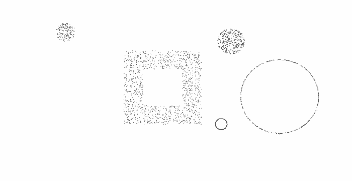
If you have a plotting package x should look like this:

Create a GrowingNeuralGasNode and train it:
>>> gng = mdp.nodes.GrowingNeuralGasNode(max_nodes=75)
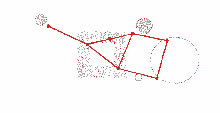
The initial distribution of nodes is randomly chosen:

The training is performed in small chunks in order to visualize the evolution of the graph:
>>> STEP = 500
>>> for i in range(0,x.shape[0],STEP):
...     gng.train(x[i:i+STEP])
...     # [...] plotting instructions
...
>>> gng.stop_training()
See The Animation of Training.
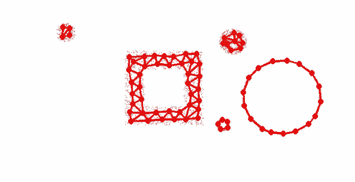
Visualizing the neural gas network, we’ll see that it is adapted to the topological structure of the data distribution:

Calculate the number of connected components:
>>> n_obj = len(gng.graph.connected_components())
>>> print n_obj
5
