Logistic Maps
CodeSnippet
You can download all the code on this page from the code snippets directory
In this example we show MDP usage in a machine learning application, and use non-linear Slow Feature Analysis for processing of non-stationary time series. We consider a chaotic time series derived by a logistic map (a demographic model of the population biomass of species in the presence of limiting factors such as food supply or disease) that is non-stationary in the sense that the underlying parameter is not fixed but is varying smoothly in time.
The goal is to extract the slowly varying parameter that is hidden in the observed time series. This example reproduces some of the results reported in Laurenz Wiskott, Estimating Driving Forces of Nonstationary Time Series with Slow Feature Analysis (arXiv.org e-Print archive).
Generate the slowly varying driving force, a combination of three sine waves (freqs: 5, 11, 13 Hz), and define a function to generate the logistic map
>>> p2 = np.pi*2
>>> t = np.linspace(0, 1, 10000, endpoint=0) # time axis 1s, samplerate 10KHz
>>> dforce = np.sin(p2*5*t) + np.sin(p2*11*t) + np.sin(p2*13*t)
>>> def logistic_map(x, r):
...     return r*x*(1-x)
Note that we define series to be a two-dimensional array.
Inputs to MDP must be two-dimensional arrays with variables
on columns and observations on rows. In this case we have only
one variable:
>>> series = np.zeros((10000, 1), 'd')
Fix the initial condition:
>>> series[0] = 0.6
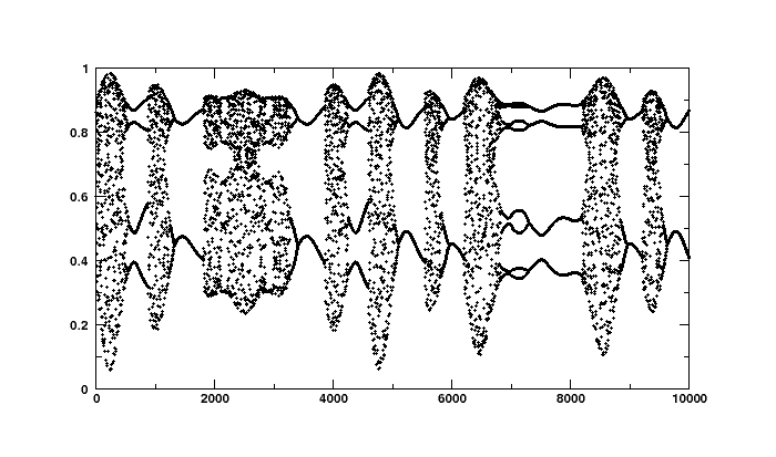
Generate the time series using the logistic equation.
The driving force modifies the logistic equation parameter r:
>>> for i in range(1,10000):
...     series[i] = logistic_map(series[i-1],3.6+0.13*dforce[i])
If you have a plotting package series should look like this:
To reconstruct the underlying parameter, we define a Flow to
perform SFA in the space of polynomials of degree 3. We first use a
node that embeds the 1-dimensional time series in a 10 dimensional
space using a sliding temporal window of size 10
(TimeFramesNode(10)). Second, we expand the signal in the space
of polynomials of degree 3 using a
PolynomialExpansionNode(3). Finally, we perform SFA on the
expanded signal and keep the slowest feature using the
SFANode(output_dim=1).
In order to measure the slowness of the input time series before and
after processing, we put at the beginning and at the end of the node
sequence a node that computes the eta-value (a measure of slowness)
of its input (EtaComputerNode()):
>>> flow = (mdp.nodes.EtaComputerNode() +
...         mdp.nodes.TimeFramesNode(10) +
...         mdp.nodes.PolynomialExpansionNode(3) +
...         mdp.nodes.SFANode(output_dim=1) +
...         mdp.nodes.EtaComputerNode() )
Since the time series is short enough to be kept in memory we don’t need to define generators and we can feed the flow directly with the whole signal:
>>> flow.train(series)
Since the second and the third nodes are not trainable we are
going to get two warnings (Training Interrupted). We can safely
ignore them. Execute the flow to get the slow feature
>>> slow = flow(series)
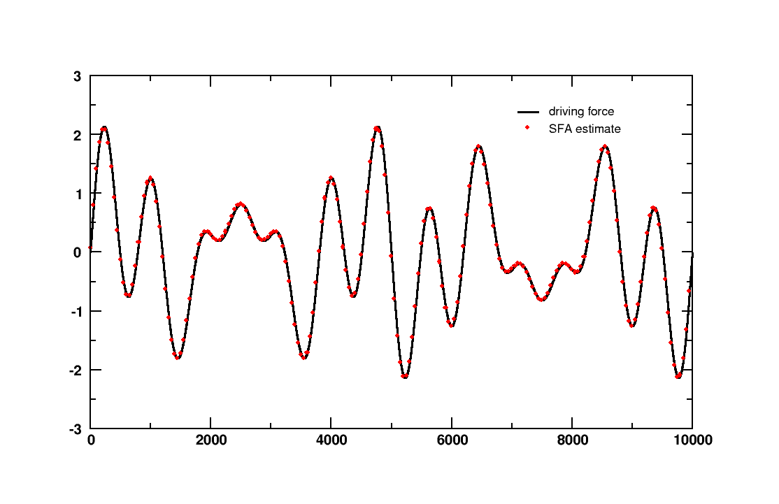
The slow feature should match the driving force up to a scaling factor, a constant offset and the sign. To allow a comparison we rescale the driving force to have zero mean and unit variance:
>>> resc_dforce = (dforce - np.mean(dforce, 0)) / np.std(dforce, 0)
Print covariance between the rescaled driving force and the slow feature. Note that embedding the time series with 10 time frames leads to a time series with 9 observations less:
>>> print '%.3f' % mdp.utils.cov2(resc_dforce[:-9], slow)
1.000
Print the eta-values of the chaotic time series and of the slow feature
>>> print 'Eta value (time series): %d' % flow[0].get_eta(t=10000)
Eta value (time series): 3004
>>> print 'Eta value (slow feature): %.3f' % flow[-1].get_eta(t=9996)
Eta value (slow feature): 10.218
If you have a plotting package you could plot the real driving force is plotted together with the driving force estimated by SFA and see that they match perfectly: