Handwritten digits classification with MDP and scikits.learn
CodeSnippet
You can download all the code on this page from the code snippets directory
If you have the library scikits.learn installed on your machine, MDP will automatically wrap the algorithms defined there, and create a new series of Nodes, whose name ends with ScikitsLearnNode.
In this example, we show how it is possible to merge MDP nodes and flows and a scikits.learn classifier to perform handwritten digit classification.
One of the nice features of scikits.learn is that it provides access to several classical dataset. First of all, we will load the digits dataset:
>>> import mdp
>>> import numpy
>>>
>>> import sklearn as sl
>>> from sklearn import datasets
>>>
>>> digits = datasets.load_digits()
>>> images = digits.images.astype('f')
>>> labels = digits.target
>>> data = digits.images.reshape((images.shape[0],
...                               numpy.prod(images.shape[1:])))
and divide it in a training and a test set:
>>> # number of digits to be used as training data (2/3 of total)
>>> ntrain = images.shape[0] // 3 * 2
>>> train_data = [data[:ntrain, :]]
>>> train_data_with_labels = [(data[:ntrain, :], labels[:ntrain])]
>>> test_data = data[ntrain:, :]
>>> test_labels = labels[ntrain:]
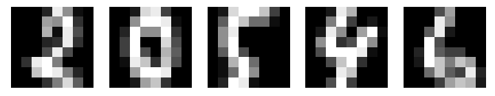
These are a few examples of the 8 x 8 images in the database:
For our handwritten digits classification application, we build a flow that performs these steps:
- reduce the dimensionality of the data from 8 x 8 = 64 to 25 using Principal Component Analysis
- expand the data in the space of polynomials of degree 3, i.e., augment the pixel data (x_1, x_2, …) with monomial of order 2 and three, like x_1 * x_2^2 or x_1 * x_3 . This is a common trick to transform a linear algorithm (in this case, the one in step 4) in a non-linear algorithm
- reduce the dimensionality of the data again, keeping 99% of the variance in the expanded data
- perform Fisher Discriminant Analysis (FDA), a supervised algorithm that finds a projection of the data that maximizes the variance between labels, and minimize the variance within labels. In other words, the algorithm tries to form well separated clusters for each label.
- classify the digit using the Support Vector Classification algorithm defined in scikits.learn
In the application, the data type is set to single precision to spare memory:
>>> flow = mdp.Flow([mdp.nodes.PCANode(output_dim=25, dtype='f'),
...                  mdp.nodes.PolynomialExpansionNode(3),
...                  mdp.nodes.PCANode(output_dim=0.99),
...                  mdp.nodes.FDANode(output_dim=9),
...                  mdp.nodes.SVCScikitsLearnNode(kernel='rbf')], verbose=True)
Note how it is possible to set parameters in the the scikits.learn algorithms simply by using the corresponding keyworg argument. In this case, we use Radial Basis Function kernels for the classifier.
We’re ready to train our algorithms on the training data set:
>>> flow.train([train_data, None, train_data,
...             train_data_with_labels, train_data_with_labels])
Training node #0 (PCANode)
Training finished
Training node #1 (PolynomialExpansionNode)
Training finished
Training node #2 (PCANode)
Training finished
Training node #3 (FDANode)
Training finished
Training node #4 (SVCScikitsLearnNode)
Training finished
Close the training phase of the last node
>>> # print the final state of the nodes
>>> print repr(flow)
Flow([PCANode(input_dim=64, output_dim=25, dtype='float32'),
      PolynomialExpansionNode(input_dim=25, output_dim=3275, dtype='float32'),
      PCANode(input_dim=3275, output_dim=646, dtype='float32'),
      FDANode(input_dim=646, output_dim=9, dtype='float32'),
      SVCScikitsLearnNode(input_dim=9, output_dim=9, dtype='float32')])
Finally, we can execute the application on the test data set, and compute the error rate:
>>> # set the execution behavior of the last node to return labels
>>> flow[-1].execute = flow[-1].label
>>>
>>> # get test labels
>>> prediction = flow(test_data)
>>> # percent error
>>> error = ((prediction.flatten() != test_labels).astype('f').sum()
...          / (images.shape[0] - ntrain) * 100.)
>>> print 'percent error:', error
percent error: 3.33889816361
One can probably do better than 3.3 percent error using a larger non-linear space, using more PCA components, or using another classifier. Have fun exploring the parameters!